When someone says Discrete Event Simulation (DES) what do you think? Technical mumbo jumbo? Actually you are used to experiencing it. It may be something you experience every day. DES is the process of breaking down continuous processes into time buckets. Within a time bucket, characteristics (or state) are represented as constant. The cause of change from one time bucket to the next is represented as discrete events.
Are you used to waking up and checking the weather for the day? What is the high and low? Will it rain, snow, be cloudy or sunny? All of these can be described characteristics (or states) of the weather in 24 hour time buckets. If you are real curious you can visit sites that will tell you the weather characteristics by the hour – just a different time bucket. The events causing temperature change from one bucket to the next are described as the delta change in pressure and humidity over the time bucket interval in the model, among others. When applied to the state of a time bucket, it creates the state for the next time bucket.
Typically you have to simulate in smaller bucket sizes than the reporting period for accuracy – as you can see below.
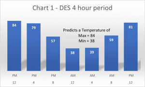
Chart 1 is simulated in 4 hour time buckets. The maximum and minimum reported temperatures are 84 and 38, respectively.
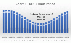
Chart 2 shows the same calculations in 1 hour time buckets. A more accurate maximum and minimum temperature pair is reported as 85 and 35, respectively.
As you simulate to smaller and smaller time buckets accuracy increases at the expense of simulation time. At some point increased accuracy will become more than required. In this example getting accuracy to hundreds of a degree does not help when you are reporting to the accuracy of 1 degree. Potentially you only need to achieve 1/2 of a degree of accuracy.
You never knew you experience Discrete Event Simulation every day.